Inputs and Outputs¶

Every Flow in Balthazar takes a set of Inputs and produces a set of Outputs. Together, they make each Run reproducible and easy to compare with other Runs.

• Inputs are the values fed into a Flow before it starts.
• Outputs are the key results the Flow produces.

Both are stored alongside the Run, so it is always clear which values were used and what came out.

---

Inputs (blt.params)¶

Inputs are the parameters of a Run. They are the dials and knobs changed between Runs, without editing the Python script.

Typical examples include:

• The start and stop voltage of a sweep, and the number of points
• The measurement mode, selected from a fixed set of options
• The averaging time in seconds for a noisy signal
• The target temperature to reach before measuring

1. Set Inputs from the interface¶

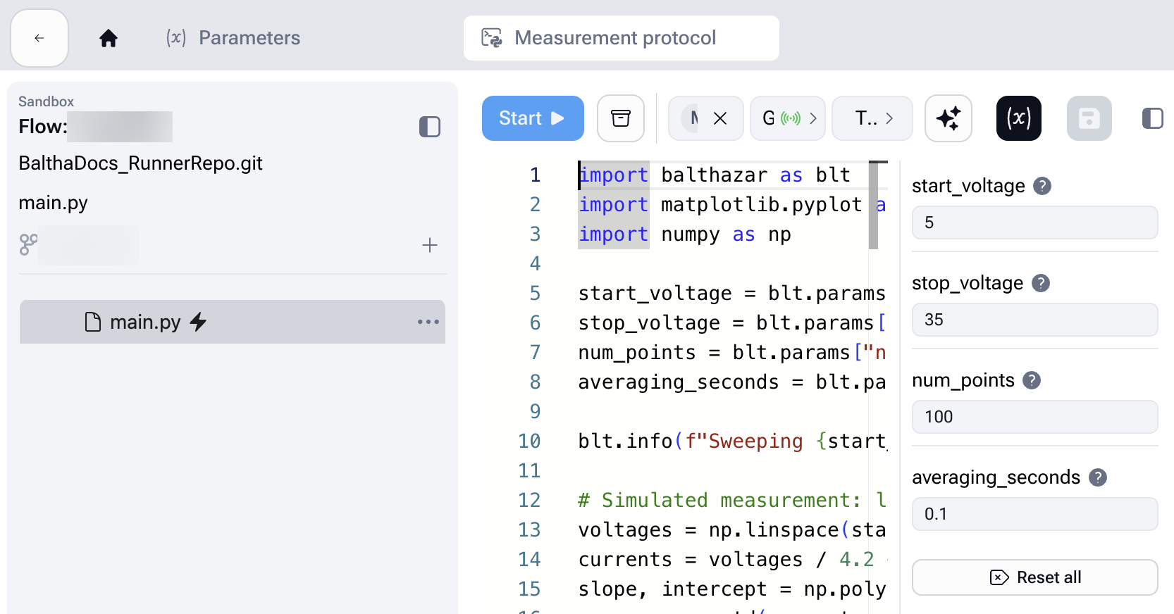
Inputs are defined once in the Workbench's Parameters tab, where each has a name, a type, and options. Their values are entered in the Parameters section of the Start dialog, each time the Flow is started.

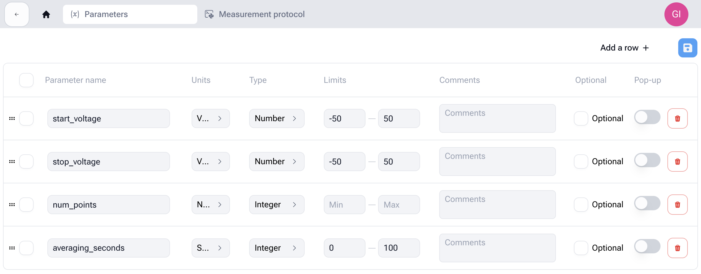
Inputs can be changed every time the Flow is started, without touching its code.

2. Give each input a type¶

Every input has a type, not just a value. The type sets which control appears in the Start dialog (a date picker, a True/False choice, or a list), so only valid values can be entered. Set each input's type, unit, and options in the Workbench's Parameters tab.

Typical types:

• Number and Integer, with optional Min and Max limits.
• Boolean, chosen as True or False.
• Date and Timestamp, shown with a picker. Time and Duration are typed in; a Duration is written like PT30M (30 minutes) or PT1H (1 hour). Time and Timestamp also come in "with timezone" variants.
• Dropdown, a fixed set of predefined choices, so a Run can only use one of them.
• Float Sweep and Integer Sweep, a range entered as Start, End, and Step. This is ideal for parameter scans such as a voltage or frequency sweep. In the Flow, an Integer Sweep arrives as a Python range (which stops before the end value), and a Float Sweep as a blt.NumberRange with .start, .end, and .step.

Each input can also carry a unit picked from the Units list (such as volt (V)), a note in the Comments column shown when the Flow is started, an Optional flag, and a Pop-up switch that asks for the value each time the Flow is started.

3. Read Inputs inside the Flow¶

Inside the Flow, import the balthazar library and read parameters from blt.params:

import balthazar as blt

# Read parameters set in the interface
start_voltage = blt.params["start_voltage"]
stop_voltage = blt.params["stop_voltage"]
num_points = blt.params["num_points"]
averaging_seconds = blt.params["averaging_seconds"]

print(f"Sweeping from {start_voltage} V to {stop_voltage} V in {num_points} points")

Each key must match an Input name in the Parameters tab.

4. Inputs are tracked with the Run¶

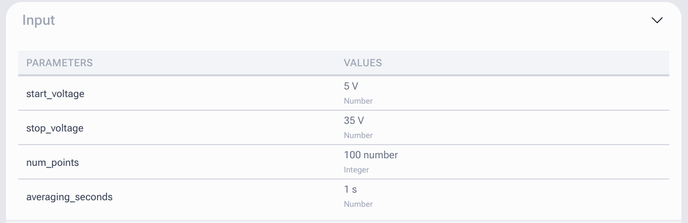
Every Run keeps the exact Inputs it used, so a past Run can be opened to check its settings or repeated with the same values.

---

Outputs (blt.output)¶

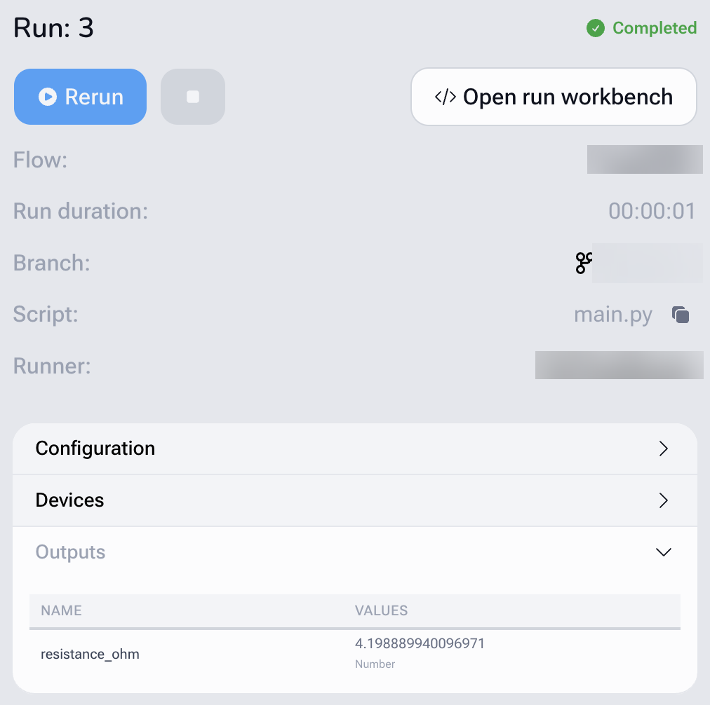
Outputs are the key results of a Run. Each Output is a key/value pair saved with blt.output["key"] = value.

A good Output is a single value, like a number or a short string, so it can be compared and aggregated across Runs. blt.output does accept lists too, but only single numbers can be aggregated across Runs.

Typical examples include:

• The resistance extracted from an I-V sweep
• The threshold voltage of a transistor
• The conversion efficiency of a solar cell
• A simple status value such as "success" or "failed"

1. Write Outputs from the Flow¶

Inside the Flow, assign values to blt.output using a key:

import balthazar as blt

# ... run the measurement and analyse it ...
peak_height = 1.42
peak_width_mhz = 3.7
center_frequency_ghz = 5.012

# Save the key results as Outputs
blt.output["peak_height"] = peak_height
blt.output["peak_width_mhz"] = peak_width_mhz
blt.output["center_frequency_ghz"] = center_frequency_ghz
blt.output["status"] = "success"

Use one key per result to track. Each assignment to blt.output is saved to the server as it happens, so write each result once rather than updating the same key over and over.

2. Outputs appear on the Run¶

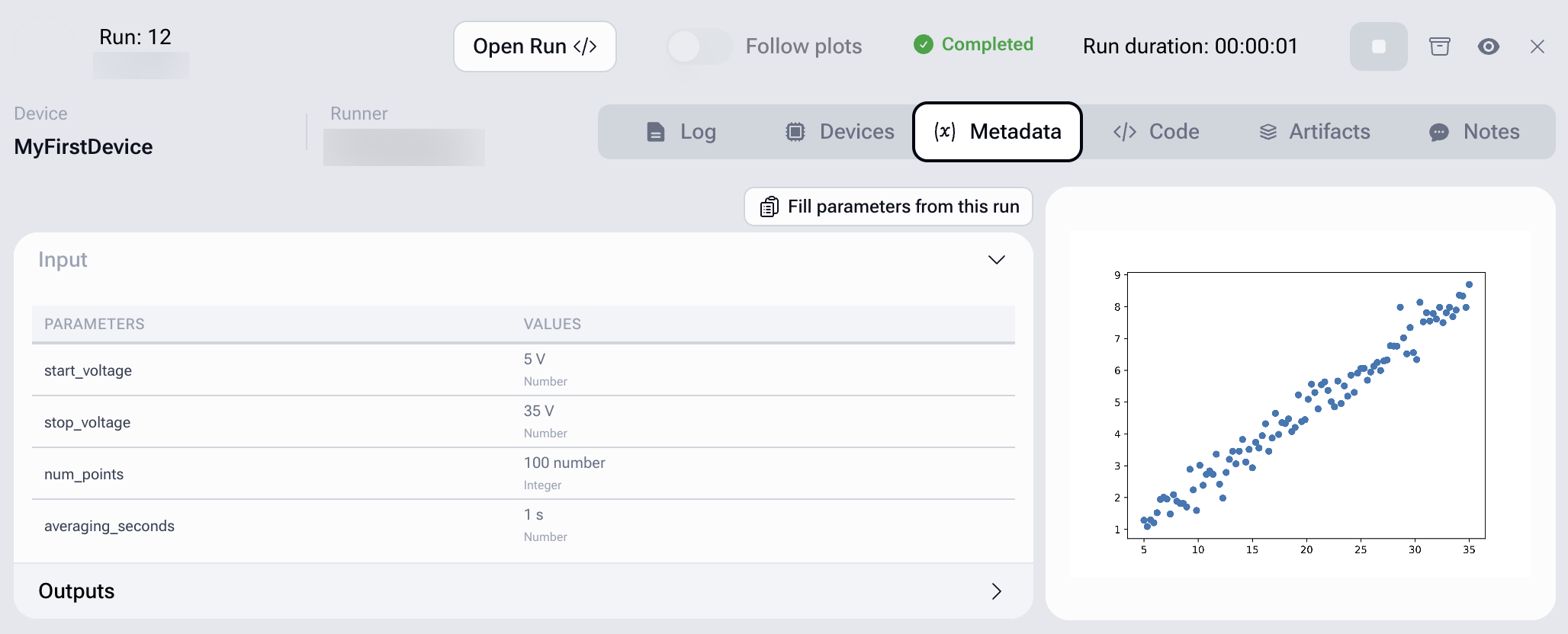
After the Flow has finished, the Outputs are visible on the Run, next to the Inputs that produced them.

3. Aggregate Outputs across Runs¶

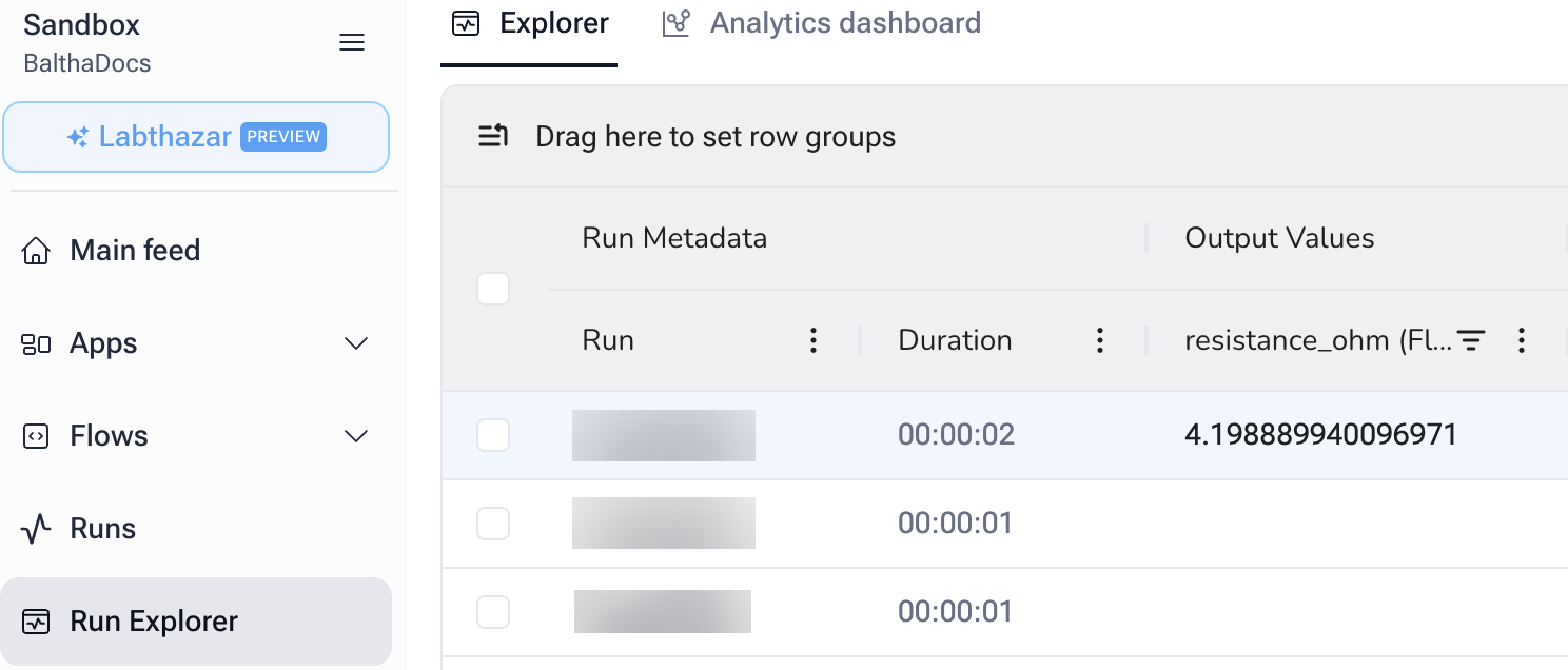
Because Outputs are typically single values, the Run Explorer can show them as columns and aggregate them across many Runs. This shows how a result evolves over many measurements (for example, resistance as a function of fabrication date, or threshold voltage across different Devices).

---

Recording files as Artifacts¶

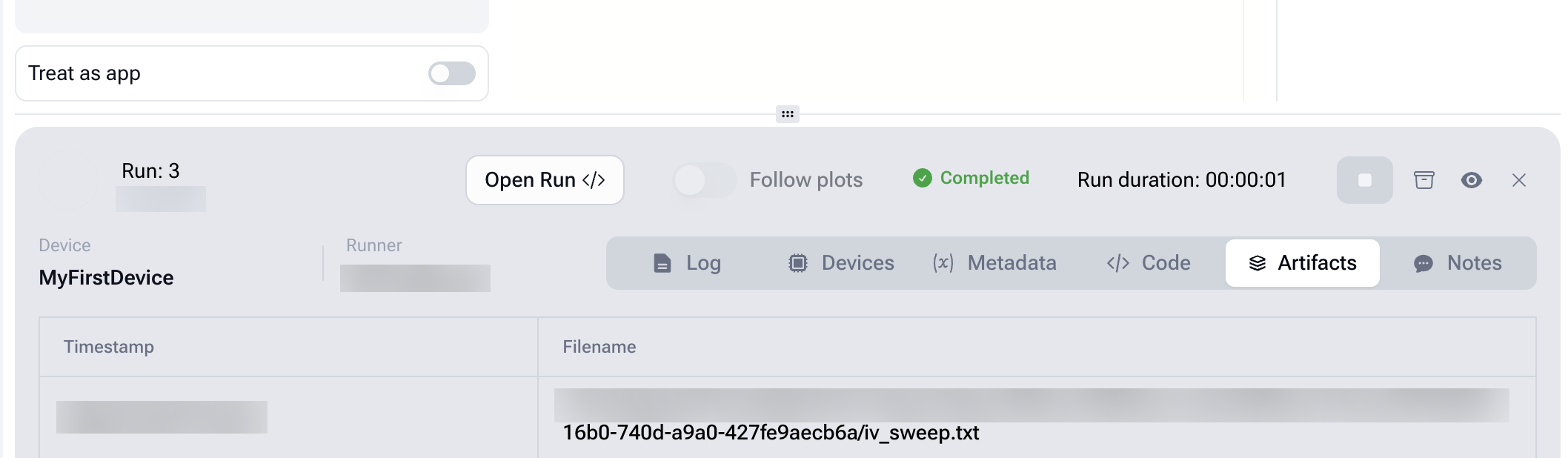
When a Flow writes a file, Balthazar records it as an Artifact on the Run: the file's name and the time it was written. This gives a record of which files each Run produced.

Balthazar records the name, not the file's contents. Use Artifacts to track what a Run wrote; save results that need comparing across Runs as Outputs (blt.output).

Example: recording a data file¶

A voltage sweep can write its raw (voltage, current) pairs to a two-column text file:

import numpy as np

# voltages and currents are arrays from the measurement loop
np.savetxt(
    "iv_sweep.txt",
    np.column_stack([voltages, currents]),
    header="voltage_V  current_A",
    comments="",
)

After the Run, iv_sweep.txt is listed in the Run's Artifacts (with its full path on the Runner's computer), recording that this Run wrote it.

---

Logs¶

In addition to print(...) (which Balthazar captures as stdout), the Balthazar SDK provides labelled log helpers that appear in the Run's log panel both during the Run and after it finishes. Five levels are available, each shown with its own coloured label:

• blt.trace(message): very fine-grained tracing, for diagnosing a specific issue.
• blt.debug(message): developer-oriented diagnostic information.
• blt.info(message): a normal informational entry, for high-level progress and key intermediate values.
• blt.warn(message): flags an unexpected condition that does not stop the Run, such as a borderline fit or a measurement that drifted out of range.
• blt.error(message): flags a problem in the log without stopping the script. It does not mark the Run as failed.

Example: logging during a sweep¶

import balthazar as blt

blt.info(f"Starting sweep from {start_voltage} V to {stop_voltage} V")

# ... measurement loop ...

if rmse_a > 1e-3:
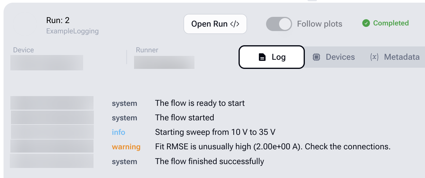
    blt.warn(f"Fit RMSE is unusually high ({rmse_a:.2e} A). Check the connections.")
else:
    blt.info(f"Fit OK. RMSE = {rmse_a:.2e} A.")

The entries appear in the Run's log panel, with warnings and errors highlighted:

---

A code migration example¶

Turning a plain script into a Flow is mostly find-and-replace:

• Parameters hard-coded at the top become Inputs: define them in the Parameters tab and read them with blt.params["name"].
• Results that are printed or returned become Outputs: save them with blt.output["key"] = value so they are searchable and comparable across Runs.
• print(...) still works and is captured in the Run's log (see Flows); for filterable messages, use blt.info, blt.warn, and blt.error.
• Files the script writes are recorded automatically as Artifacts (by name), with no change needed.

A plain script that runs a noisy I-V sweep, fits the resistance, and saves the raw data:

# Before: a plain script
import numpy as np

max_voltage = 0.5
num_points = 50

voltages = np.linspace(0, max_voltage, num_points)
currents = voltages / 4.2 + np.random.normal(0, 1e-3, num_points)  # noisy 4.2 ohm resistor
resistance = 1 / np.polyfit(voltages, currents, 1)[0]

np.savetxt("iv_sweep.txt", np.column_stack([voltages, currents]))
print(f"Resistance: {resistance:.2f} Ohm")

The same script as a Flow. Add max_voltage (Number) and num_points (Integer) in the Parameters tab, then paste it into a Flow and start it:

# After: the same script as a Flow
import balthazar as blt
import numpy as np

max_voltage = blt.params["max_voltage"]
num_points = blt.params["num_points"]

blt.info(f"Sweeping 0 to {max_voltage} V in {num_points} points")  # progress log via blt.info

voltages = np.linspace(0, max_voltage, num_points)
currents = voltages / 4.2 + np.random.normal(0, 1e-3, num_points)  # noisy 4.2 ohm resistor
resistance = 1 / np.polyfit(voltages, currents, 1)[0]

np.savetxt("iv_sweep.txt", np.column_stack([voltages, currents]))  # unchanged; recorded as an Artifact (name only)
blt.output["resistance_ohm"] = float(resistance)  # the searchable key result

---

Complete example¶

A runnable Flow using everything on this page. It simulates an I-V sweep of a 4.2 ohm resistor, so no instrument is needed. It reads four Inputs: start_voltage and stop_voltage (V), num_points (Integer), and averaging_seconds (s).

import balthazar as blt
import matplotlib.pyplot as plt
import numpy as np

start_voltage = blt.params["start_voltage"]
stop_voltage = blt.params["stop_voltage"]
num_points = blt.params["num_points"]
averaging_seconds = blt.params["averaging_seconds"]

blt.info(f"Sweeping {start_voltage} to {stop_voltage} V in {num_points} points")

# Simulated measurement: noise is 5 % of full scale at 1 s averaging
voltages = np.linspace(start_voltage, stop_voltage, num_points)
full_scale_a = stop_voltage / 4.2
noise_a = 0.05 * full_scale_a / np.sqrt(averaging_seconds)
currents = voltages / 4.2 + np.random.normal(0, noise_a, num_points)
slope, intercept = np.polyfit(voltages, currents, 1)
rmse_a = np.std(currents - (slope * voltages + intercept))

plt.plot(voltages, currents, "o")
plt.show()  # captured as a plot

np.savetxt("iv_sweep.txt", np.column_stack([voltages, currents]))  # recorded as an Artifact

if rmse_a > 0.1 * full_scale_a:
    blt.warn(f"Noisy fit (RMSE {rmse_a:.1e} A). Try a longer averaging time.")

blt.output["resistance_ohm"] = float(1 / slope)  # about 4.2

With averaging_seconds at 1 the fit is clean; at 0.1 the warning appears in the log.